
Exploring Hough Transform with Floor Detection: My journey
When it comes to image processing, detecting boundaries and structures from images is crucial, especially for tasks like helping robots navigate through rooms. Imagine trying to identify the floor’s edges from a complex room layout, this is where the Hough Transform comes into play.
Hough Transform is an amazing technique used in image processing to find shapes, like straight lines, circles, and ellipses within an image. For this project, it helped me find the straight edges of the floor in the image, which is essential for detecting its boundaries.
In this post, I’ll take you through the exciting journey of using this powerful technique to detect the floor in a top-view image of a room. So, let’s dive in and explore how the Hough Transform helped me detect the floor, step by step.
The Process
1. Loading the Image

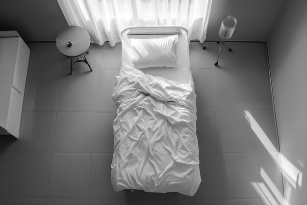
I started by loading my test image, the image above which is a top-view image of a room. To make the image simpler to work with, I converted it to grayscale (black and white) making it easier to focus on the important features of the image.
import cv2

# Load image and convert to grayscale
image = cv2.imread('topdown.jpg')
gray = cv2.cvtColor(image, cv2.COLOR_BGR2GRAY)
cv2.imwrite('grayscale.png', gray)
Result Image:
2. Blurring the Image
Next, I blurred the image a little to remove noise from it. Noise can cause false edges, so the blur helps by smoothing out the image.
# Apply Gaussian Blur
blurred = cv2.GaussianBlur(gray, (5, 5), 0)
cv2.imwrite('blurred.png', blurred)
Result Image:

3. Detecting Edges
To find the edges, I used the Canny edge detector.
What is the Canny Edge Detector?
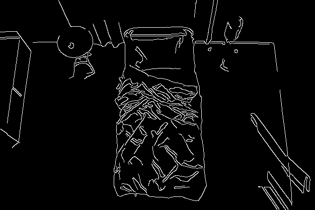
The Canny Edge Detector is an algorithm used to detect edges in an image. It works by looking for areas in the image where the color intensity changes sharply, such as where an object’s outline meets a background. These sharp changes are the “edges” we want to highlight.
This algorithm looks for sharp changes in the image (edges) and highlights them, making it easier to find where the floor’s boundary is.
# Perform Canny Edge Detection
edges = cv2.Canny(blurred, 50, 150)
cv2.imwrite('edges.png', edges)
Result Image:
4. Detect Lines with Hough Transform
Hough Transform is a key technique that permitted me to identify straight lines in the image. These lines represent the boundaries of the floor or walls that will help us identify the layout.
It transforms points in the image from Cartesian coordinates (x, y) to a parameter space known as the Hough space (M-C space). This transformation helps group points that lie along the same line in the XY plane.
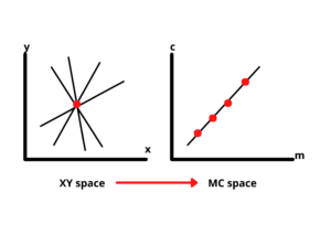
To detect lines, we look for intersections in the Hough space. If two or more lines intersect, it means their corresponding points on the XY plane belong to the same line.
The process involves identifying potential lines from points in the gradient image. However, to properly define these lines, we need their specific parameters.
We divide the Hough space into a grid of small squares to find these parameters. The square with the most intersections indicates the best values for cc (intercept) and mm (slope), which we then use to draw the most accurate line (Best fit line).
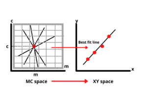
This method works well for lines with a defined slope. However, vertical lines pose a challenge because their slope is undefined (infinite). To handle this, we adopt a different approach.
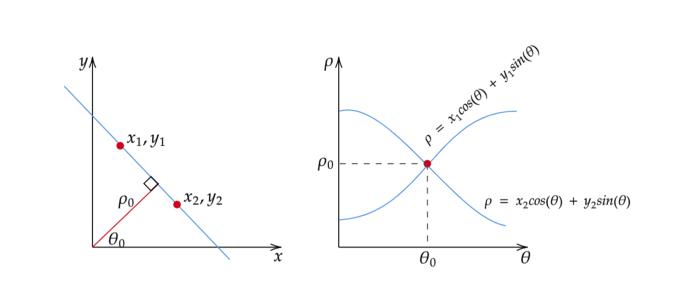
Rather than using the equation y=mx+cy = mx + cy=mx+c, we represent the line in polar coordinates as:
ρ = Xcosθ+Ysinθ
Where:
- rho(ρ): the perpendicular distance from the origin to the line.
- theta(θ): the angle between the line’s normal and the x-axis.
This adjustment allows us to accurately represent all types of lines, including vertical ones.

When a line is represented in polar coordinates, it appears as a sinusoidal curve in the Hough space rather than a straight line.
Each point generates a curve based on the different ρ and θ values for the lines passing through it. With more points, more curves are formed in the Hough space. As before, the point where the most curves intersect provides the values needed to determine the best fit line.
i. Applying the Hough Transform:
lines = cv2.HoughLines(edges, 1, np.pi / 180, threshold=100)

line_image = np.copy(image)
we use OpenCV’s HoughLines function to detect lines in the edge-detected image. The parameters passed to the function are:
- edges: The image with edges detected by the Canny algorithm.
- 1: The distance resolution of the accumulator (in pixels). In other words, it determines how finely we sample the distance between lines.
- np.pi / 180: The angle resolution of the accumulator (in radians). This specifies how finely we sample the angle between lines.
- threshold=100: This is the minimum number of intersections required in the accumulator for a line to be considered a valid detection. A higher threshold value means fewer lines will be detected, but they will likely be more robust.
We make a copy of the original image so that we can draw the detected lines without modifying the original.
ii. Converting the Polar Coordinates Back to Cartesian Coordinates:
for rho, theta in lines[:, 0]:
    a = np.cos(theta)
    b = np.sin(theta)
    x0 = a * rho
    y0 = b * rho
    x1 = int(x0 + 1000 * (-b))
    y1 = int(y0 + 1000 * (a))
    x2 = int(x0 - 1000 * (-b))
    y2 = int(y0 - 1000 * (a))


cv2.line(line_image, (x1, y1), (x2, y2), (0, 255, 0), 1)

cv2.imwrite('HoughLines.png', line_image)
Each line is represented by polar coordinates ρρ and θθ. To draw the line in the Cartesian space (image coordinates), we need to convert the polar coordinates back to Cartesian coordinates. This is done using the following steps:
- a and b are the cosine and sine of the angle θθ, respectively, which represent the direction of the line.
- x0, y0 are the coordinates of the point on the line that is at a perpendicular distance of ρρ from the origin.
- x1, y1, and x2, y2 are the endpoints of the line, which are calculated by extending the line far in both directions. The factor of 1000 ensures that the line is drawn long enough to cover the image.
- cv2.line() function, we draw each detected line on the line_image. The lines are drawn in green with a thickness of 1 pixel
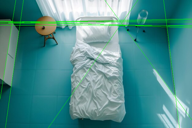
Result Image: The straight lines found by the Hough Transform are drawn in green, showing where the boundaries might be.

5. Finding Where the Lines Intersect
After detecting the lines, the next step is to find where the lines intersect. These intersections can help us find the corners of the floor.
I iterated through the lines to calculate intersections. If two lines intersect within the image bounds, I consider it a candidate corner. This gave me a list of intersection points that could be potential corners of the floor.
def get_intersection(line1, line2):
    rho1, theta1 = line1
    rho2, theta2 = line2
    a1, b1 = np.cos(theta1), np.sin(theta1)
    a2, b2 = np.cos(theta2), np.sin(theta2)

    # Solve linear equations to find intersection
    determinant = a1 * b2 - a2 * b1
    if abs(determinant) < 1e-5:
        return None  # Lines are parallel

    x = (b2 * rho1 - b1 * rho2) / determinant
    y = (a1 * rho2 - a2 * rho1) / determinant
    return (x, y)
6. Scoring the Best Floor Boundary
Finally, I generated possible quadrilaterals (4-corner shapes) using the intersection points. I then scored each quadrilateral based on how well it aligned with the edges of the image. The shape with the best score was selected as the floor boundary.
After scoring all possible quadrilaterals, I picked the one that best matched the floor edges.
def score_quadrilateral(quadrilateral, edges):
    score = 0
    for point in quadrilateral:
        x, y = point
        if 0 <= int(x) < edges.shape[1] and 0 <= int(y) < edges.shape[0]:
            score += edges[int(y), int(x)]
    return score
7. Displaying the Final Result
After finding the best quadrilateral, I drew it on the image to highlight the detected floor area.
if best_quadrilateral is not None:
    best_quadrilateral = np.array(best_quadrilateral, dtype=np.int32)
    cv2.polylines(image, [best_quadrilateral], isClosed=True, color=(255, 0, 0), thickness=2)

cv2.imwrite('detected_floor.png', image)
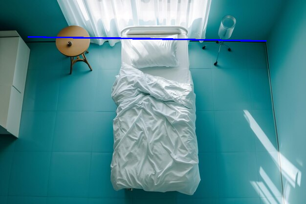
Result Image: The floor boundary is marked in blue.
The Challenge
While the results were interesting, they weren’t perfect. The final output didn’t detect the floor as accurately as I’d hoped. There are still some challenges, like misaligned corners and incomplete edges. I believe there’s room for improvement, and I’d love to hear suggestions from others who have worked with similar image-processing problems.
Looking for Help
If anyone has experience with Hough Transform or floor detection in top-view images, I’d really appreciate your feedback.
Any tips or insights on how to improve accuracy would be greatly valued.
